# mathematical functions with numbers
log(10)
[1] 2.302585# average a range of numbers
mean(1:5)[1] 3[1] 3# functions with characters
print("Hello World")[1] "Hello World"paste("Hello", "World", sep = "-")[1] "Hello-World"In this lesson we will get a general introduction to coding in RStudio, using R Markdown, some R fundamentals such as data types and indexing, and touch on a range of coding topics that we will dive into deeper throughout the course.
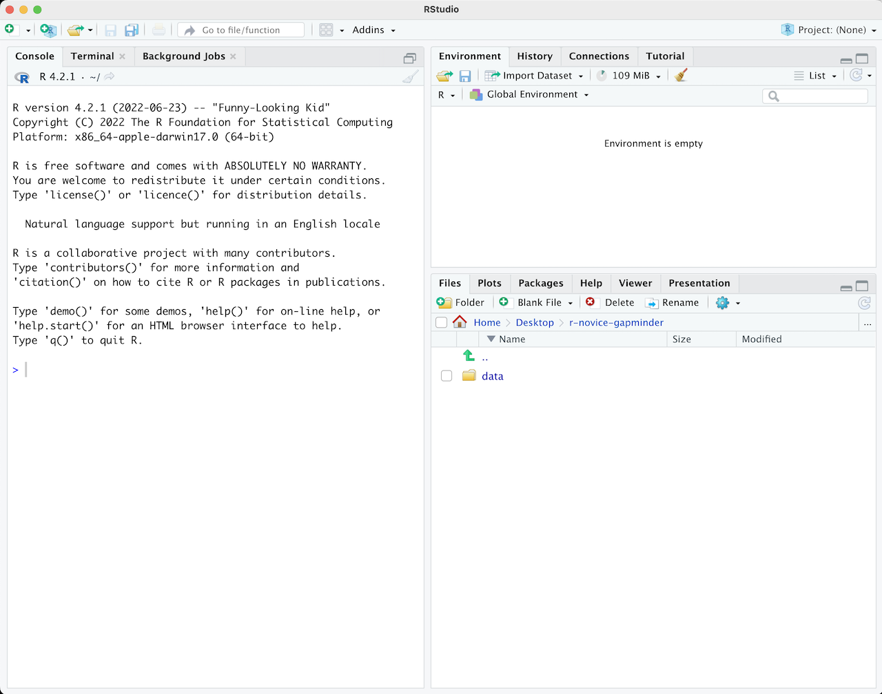
When you first open RStudio, it is split into 3 panels:
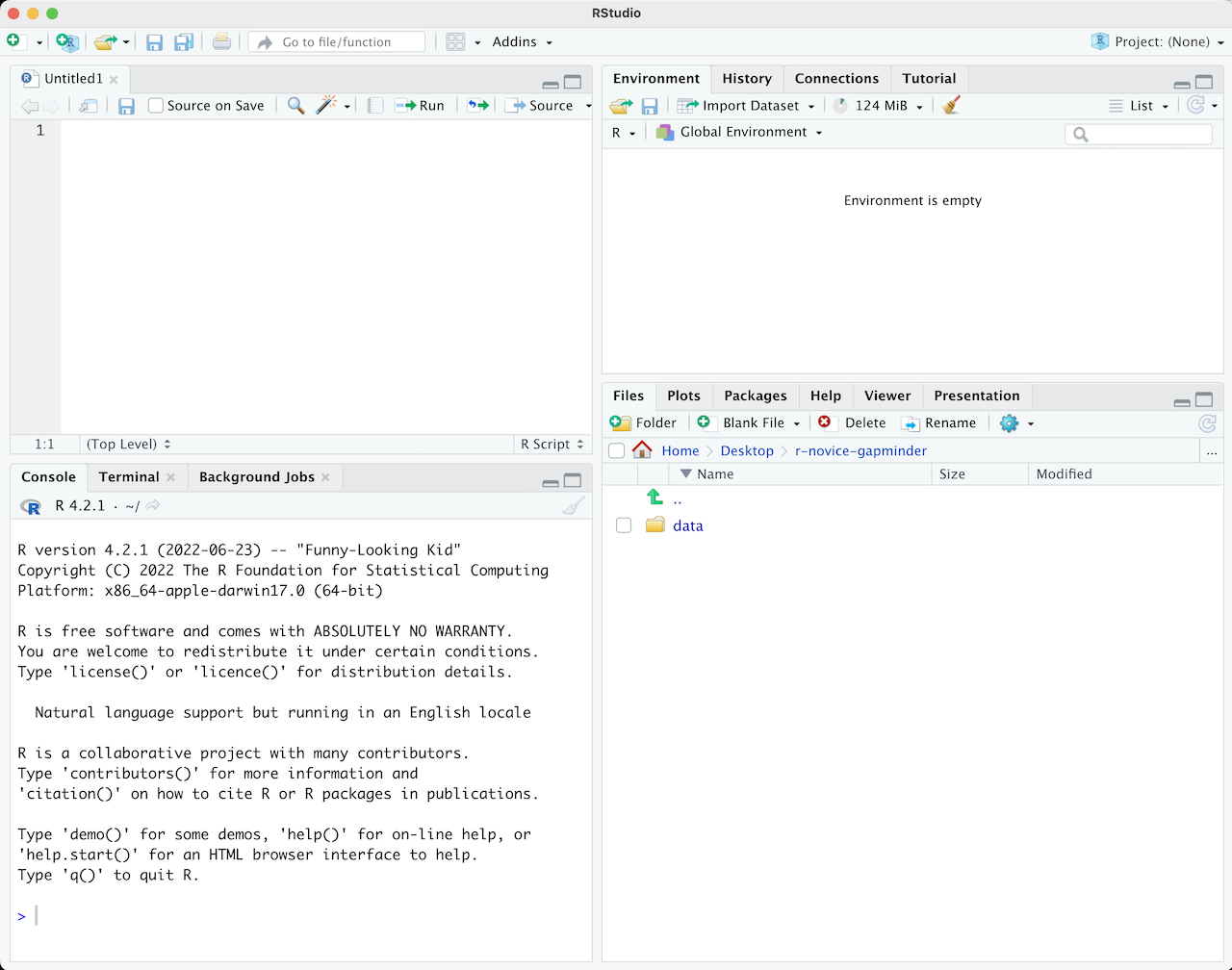
To write and save code you use .R scripts (or RMarkdown, which we will learn shortly). You can open a new script with File -> New File or by clicking the icon with the green plus sign in the upper left corner. When you open a script, RStudio then opens a fourth ‘Source’ panel in the upper-left to write and save your code. You can also send code from a script directly to the console to execute it by highlighting the entire code line/chunk (or place your cursor at the end of the code chunk) and hit CTRL+ENTER on a PC or CMD+ENTER on a Mac.
It is good practice to add comments/notes throughout your scripts to document what the code is doing. To do this start a line with a #. R knows to ignore everything after a #, so you can write whatever you want there. Note that R reads line by line, so if you want your comments to carry over multiple lines you need a # at every line.
As a first step whenever you start a new project, workflow, analysis, etc., it is good practice to set up an R project. R Projects are RStudio’s way of bundling together all your files for a specific project, such as data, scripts, results, figures. Your project directory also becomes your working directory, so everything is self-contained and easily portable.
We recommend using a single R Project (i.e., contained in a single folder) for this course, so lets create one now.
You can start an R project in an existing directory or in a new one. To create a project go to File -> New Project:
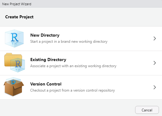
Let’s choose ‘New Directory’ then ‘New Project’. Now choose a directory name, this will be both the folder name and the project name, so use proper spelling conventions (no spaces!). We recommend naming it something course specific, like ‘WR-696-2023’, or even more generic ‘Intro-R-Fall23’. Choose where on your local file system you want to save this new folder/project (somewhere you can find it easily), then click ‘Create Project’.
Now you can see your RStudio session is working in the R project you just created. You can see the working directory printed at the top of your console is now the project directory, and in the ‘Files’ tab in RStudio you can see there is an .Rproj file with the same name as the R project, which will open up this R project in RStudio whenever you come back to it.
Test out how this .Rproj file works. Close out of your R session, navigate to the project folder on your computer, and double-click the .Rproj file.
What is a working directory? A working directory is the default file path to a specific file location on your computer to read files from or save files to. Since everyone’s computer is unique, everyone’s full file paths will be different. This is an advantage of working in R Projects, you can use relative file paths, since the working directory defaults to wherever the .RProj file is saved on your computer you don’t need to specify the full unique path to read and write files within the project directory.
HIGHLY Recommended Review: Understanding of file management is essential, especially when we start working in Git and GitHub later on. Please review these two videos:
File Paths and R Projects: https://www.youtube.com/watch?v=lJcuXBFP7Co
General File Management on Mac and PC: https://www.youtube.com/watch?v=DGd48PGbnBs
Let’s start coding!
The first thing you do in a fresh R session is set up your environment, which mostly includes installing and loading necessary libraries and reading in required data sets. Let’s open a fresh R script and save it in our root (project) directory. Call this script ‘setup.R’.
Before creating a set up script, it might be helpful to understand the use of functions in R if you are new to this programming language. R has many built-in functions to perform various tasks. To run these functions you type the function name followed by parentheses. Within the parentheses you put in your specific arguments needed to run the function.
R Packages include reusable functions that are not built-in with R. To use these functions, you must install the package to your local system with the install.packages() function. Once a package is installed on your computer you don’t need to install it again (you will likely need to update it at some point though). Anytime you want to use the package in a new R session you load it with the library() function.
When do I use :: ?
If you have a package installed, you don’t necessarily have to load it in with library() to use it in your R session. Instead, you can type the package name followed by :: and use any functions in that package. This may be useful for some one-off functions using a specific package, however if you will be using packages a lot throughout your workflow you will want to load it in to your session. You should also use :: in cases where you have multiple packages loaded that may have conflicting functions (e.g., plot() in Base R vs. plot() in the {terra} package).
You may hear us use the terms ‘Base R’ and ‘Tidyverse’ a lot throughout this course. Base R includes functions that are installed with the R software and do not require the installation of additional packages to use them. The Tidyverse is a collection of R packages designed for data manipulation, exploration, and visualization that you are likely to use in every day data analysis, and all use the same design philosophy, grammar, and data structures. When you install the Tidyverse, it installs all of these packages, and you can then load all of them in your R session with library(tidyverse). Base R and the Tidyverse have many similar functions, but many prefer the style, efficiency and functionality of the Tidyverse packages, and we will mostly be sticking to Tidyverse functions for this course.
To make code reproducible (meaning anyone can run your code from their local machines) we can write a function that checks whether or not necessary packages are installed, if not install them and load them, or if they are already installed it will only load them and not re-install. This function looks like:
packageLoad <-
  function(x) {
    for (i in 1:length(x)) {
      if (!x[i] %in% installed.packages()) {
        install.packages(x[i])
      }
      library(x[i], character.only = TRUE)
    }
  }
For each package name given (‘x’) it checks if it is already installed, if not installs it, and then loads that package into the session. In future lessons we will learn more about writing custom functions, and iterating with for loops, but for now you can copy/paste this function and put it at the top of your set up script. When you execute this chunk of code, you won’t see anything printed in the console, however you should now see packageLoad() in your Environment under ‘Functions’. You can now use this function as many times as you want. Test is out, and use it to install the Tidyverse package(s).
packageLoad('tidyverse')You can also give this function a string of package names. Lets install all the packages we will need for the first week, or if you already followed the set up instructions, this will just load the packages into your session since you already installed them.
# create a string of package names
packages <- c('tidyverse',
              'palmerpenguins',
              'rmarkdown')
# use the packageLoad function we created on those packages
packageLoad(packages)
Since this is code you will be re-using throughout your workflows, we will save it as its own script and run it at the beginning of other scripts/documents using the source() function as a part of our reproducible workflows.
Throughout this course you will be working mostly in R Markdown documents. R Markdown is a notebook style interface integrating text and code, allowing you to create fully reproducible documents and render them to various elegantly formatted static or dynamic outputs (which is how you will be submitting your assignments).
You can learn more at the R Markdown website, which has really informative lessons on the Getting Started page and you can see the range of outputs you can create at the Gallery page.
Some of you may have heard of Quarto, which is essentially an extension of R Markdown but it lives as its own software to allow its use in other languages such as Python, Julia and Observable. You can install the Quarto CLI on its own and RStudio will detect it so you can create documents within the IDE, but with current versions of RStudio a version of Quarto is built-in and you can enable Quarto through the R Markdown tab in Global Options. R Markdown isn’t going anywhere, however many in the data science realm are switching to Quarto. Quarto documents are very similar to R Markdown, in fact Quarto can even render R Markdown documents, so after learning R Markdown in this course you should have some of the fundamental skills to easily switch to Quarto if you want to. You can read more about Quarto here.
Let’s create a new document by going to File -> New File -> R Markdown. You will be prompted to add information like title and author, fill those in (let’s call it “Intro to R and R Markdown”) and keep the output as HTML for now. Click OK to create the document.
This creates an outline of an R Markdown document, and you see the title, author and date you gave the prompt at the top of the document which is called the YAML header.
Notice that the file contains three types of content:
An (optional) YAML header surrounded by ---s
R code chunks surrounded by ```s
text mixed with simple text formatting
Since this is a notebook style document, you run the code chunks by clicking the green play button in the top right corner of each code chunk, and then the output is returned directly below the chunk.
If you’d rather have the code chunk output go to the console instead of directly below the chunk in your R Markdown document, go to Tools -> Global Options -> R Markdown and uncheck “Show output inline for all R Markdown documents”
When you want to create a report from your notebook, you render it by hitting the ‘knit’ button at the top of the Source pane (with the ball of yarn next to it), and it will render to the format you have specified in the YAML header. In order to do so though, you need to have the {rmarkdown} package installed.
You can delete the rest of the code/text below the YAML header, and insert a new code chunk at the top. You can insert code chunks by clicking the green C with the ‘+’ sign at the top of the source editor, or with the keyboard short cut (Ctrl+Alt+I for Windows, Option+Command+I for Macs). For the rest of the lesson (and course) you will be writing and executing code through code chunks, and you can type any notes in the main body of the document.
The first chunk is almost always your set up code, where you read in libraries and any necessary data sets. Here we will execute our set up script to install and load all the libraries we need:
source("setup.R")Normally when working with a new data set, the first thing we do is explore the data to better understand what we’re working with. To do so, you also need to understand the fundamental data types and structures you can work with in R.
penguins dataFor this intro lesson, we are going to use the Palmer Penguins data set (which is loaded with the {palmerpenguins} package you installed in your set up script). This data was collected and made available by Dr. Kristen Gorman and the Palmer Station, Antarctica LTER, a member of the Long Term Ecological Research Network.
Load the penguins data set.
data("penguins")You now see it in the Environment pane. Print it to the console to see a snapshot of the data:
penguins# A tibble: 344 × 8
species island bill_length_mm bill_depth_mm flipper_length_mm body_mass_g
<fct> <fct> <dbl> <dbl> <int> <int>
1 Adelie Torgersen 39.1 18.7 181 3750
2 Adelie Torgersen 39.5 17.4 186 3800
3 Adelie Torgersen 40.3 18 195 3250
4 Adelie Torgersen NA NA NA NA
5 Adelie Torgersen 36.7 19.3 193 3450
6 Adelie Torgersen 39.3 20.6 190 3650
7 Adelie Torgersen 38.9 17.8 181 3625
8 Adelie Torgersen 39.2 19.6 195 4675
9 Adelie Torgersen 34.1 18.1 193 3475
10 Adelie Torgersen 42 20.2 190 4250
# ℹ 334 more rows
# ℹ 2 more variables: sex <fct>, year <int>This data is structured as a data frame, probably the most common data type and one you are most familiar with. These are like Excel spreadsheets: tabular data organized by rows and columns. However we see at the top this is called a tibble which is just a fancy kind of data frame specific to the Tidyverse.
At the top we can see the data type of each column. There are five main data types:
character: "a", "swc"
numeric: 2, 15.5
integer: 2L (the L tells R to store this as an integer)
logical: TRUE, FALSE
complex: 1+4i (complex numbers with real and imaginary parts)
Data types are combined to form data structures. R’s basic data structures include:
atomic vector
list
matrix
data frame
factors
You can see the data type or structure of an object using the class() function, and get more specific details using the str() function. (Note that ‘tbl’ stands for tibble).
class(penguins)[1] "tbl_df" "tbl" "data.frame"str(penguins)tibble [344 × 8] (S3: tbl_df/tbl/data.frame)
$ species : Factor w/ 3 levels "Adelie","Chinstrap",..: 1 1 1 1 1 1 1 1 1 1 ...
$ island : Factor w/ 3 levels "Biscoe","Dream",..: 3 3 3 3 3 3 3 3 3 3 ...
$ bill_length_mm : num [1:344] 39.1 39.5 40.3 NA 36.7 39.3 38.9 39.2 34.1 42 ...
$ bill_depth_mm : num [1:344] 18.7 17.4 18 NA 19.3 20.6 17.8 19.6 18.1 20.2 ...
$ flipper_length_mm: int [1:344] 181 186 195 NA 193 190 181 195 193 190 ...
$ body_mass_g : int [1:344] 3750 3800 3250 NA 3450 3650 3625 4675 3475 4250 ...
$ sex : Factor w/ 2 levels "female","male": 2 1 1 NA 1 2 1 2 NA NA ...
$ year : int [1:344] 2007 2007 2007 2007 2007 2007 2007 2007 2007 2007 ...class(penguins$species)[1] "factor"str(penguins$species) Factor w/ 3 levels "Adelie","Chinstrap",..: 1 1 1 1 1 1 1 1 1 1 ...When we pull one column from a data frame like we just did above using the $ operator, that returns a vector. Vectors are 1-dimensional, and must contain data of a single data type (i.e., you cannot have a vector of both numbers and characters).
If you want a 1-dimensional object that holds mixed data types and structures, that would be a list. You can put together pretty much anything in a list.
List of 4
$ : chr "apple"
$ : num 1993
$ : logi FALSE
$ : tibble [344 × 8] (S3: tbl_df/tbl/data.frame)
..$ species : Factor w/ 3 levels "Adelie","Chinstrap",..: 1 1 1 1 1 1 1 1 1 1 ...
..$ island : Factor w/ 3 levels "Biscoe","Dream",..: 3 3 3 3 3 3 3 3 3 3 ...
..$ bill_length_mm : num [1:344] 39.1 39.5 40.3 NA 36.7 39.3 38.9 39.2 34.1 42 ...
..$ bill_depth_mm : num [1:344] 18.7 17.4 18 NA 19.3 20.6 17.8 19.6 18.1 20.2 ...
..$ flipper_length_mm: int [1:344] 181 186 195 NA 193 190 181 195 193 190 ...
..$ body_mass_g : int [1:344] 3750 3800 3250 NA 3450 3650 3625 4675 3475 4250 ...
..$ sex : Factor w/ 2 levels "female","male": 2 1 1 NA 1 2 1 2 NA NA ...
..$ year : int [1:344] 2007 2007 2007 2007 2007 2007 2007 2007 2007 2007 ...You can even nest lists within lists:
[[1]]
[[1]][[1]]
[1] "apple"
[[1]][[2]]
[1] 1993
[[1]][[3]]
[1] FALSE
[[1]][[4]]
# A tibble: 344 × 8
   species island    bill_length_mm bill_depth_mm flipper_length_mm body_mass_g
   <fct>   <fct>              <dbl>         <dbl>             <int>       <int>
 1 Adelie  Torgersen           39.1          18.7               181        3750
 2 Adelie  Torgersen           39.5          17.4               186        3800
 3 Adelie  Torgersen           40.3          18                 195        3250
 4 Adelie  Torgersen           NA            NA                  NA          NA
 5 Adelie  Torgersen           36.7          19.3               193        3450
 6 Adelie  Torgersen           39.3          20.6               190        3650
 7 Adelie  Torgersen           38.9          17.8               181        3625
 8 Adelie  Torgersen           39.2          19.6               195        4675
 9 Adelie  Torgersen           34.1          18.1               193        3475
10 Adelie  Torgersen           42            20.2               190        4250
# ℹ 334 more rows
# ℹ 2 more variables: sex <fct>, year <int>
[[2]]
[[2]][[1]]
[1] "more stuff here"
[[2]][[2]]
[[2]][[2]][[1]]
[1] "and more"You can use the names() function to retrieve or assign names to list and vector elements:
Indexing is an extremely important aspect to data exploration and manipulation. In fact you already started indexing when we looked at the data type of individual columns with penguins$species. How you index is dependent on the data structure.
Index lists:
# for lists we use double brackes [[]]
myList[[1]] # select the first stored object in the list
[1] "apple"myList[["data"]] # select the object in the list named "data" (a data frame)# A tibble: 344 × 8
species island bill_length_mm bill_depth_mm flipper_length_mm body_mass_g
<fct> <fct> <dbl> <dbl> <int> <int>
1 Adelie Torgersen 39.1 18.7 181 3750
2 Adelie Torgersen 39.5 17.4 186 3800
3 Adelie Torgersen 40.3 18 195 3250
4 Adelie Torgersen NA NA NA NA
5 Adelie Torgersen 36.7 19.3 193 3450
6 Adelie Torgersen 39.3 20.6 190 3650
7 Adelie Torgersen 38.9 17.8 181 3625
8 Adelie Torgersen 39.2 19.6 195 4675
9 Adelie Torgersen 34.1 18.1 193 3475
10 Adelie Torgersen 42 20.2 190 4250
# ℹ 334 more rows
# ℹ 2 more variables: sex <fct>, year <int>Index vectors:
# for vectors we use single brackets []
myVector <- c("apple", "banana", "pear")
myVector[2]
[1] "banana"Index data frames:
# dataframe[row(s), columns()]
penguins[1:5, 2]

penguins[1:5, "island"]

penguins[1, 1:5]

penguins[1:5, c("species","sex")]

penguins[penguins$sex=='female',]

# $ for a single column
penguins$species
To index elements of a list you must use double brackets [[ ]], and to index vectors and data frames you use single brackets [ ]
We used an R data package today to read in our data frame, but that probably isn’t how you will normally read in your data.
There are many ways to read and write data in R. To read in .csv files, you can use read_csv() which is included in the Tidyverse with the {readr} package, and to save csv files use write_csv(). The {readxl} package is great for reading in excel files, however it is not included in the Tidyverse and will need to be loaded separately.
(not required, but highly recommended!)
Use indexing to create a new data frame called chinstrap_data that contains only Chinstrap penguins and includes all columns. How many Chinstrap penguins are in the dataset? (Hint: use nrow() or dim()).
What is the maximum body mass recorded for penguins on Biscoe island? Use indexing and the max() function to find out. (Hint: remember to handle NA values with na.rm = TRUE).
Create a vector called male_species that contains only the species names for all male penguins in the dataset. Use the unique() function to see which species the males belong to.
Use indexing to find the bill length (bill_length_mm) of the penguin in row 15. Then find all penguins that have a bill length greater than this value. How many are there?
Create a new data frame called dream_summary that contains only penguins from Dream island and only these four columns: species, bill_length_mm, bill_depth_mm, and body_mass_g. Then calculate the average bill depth for these Dream island penguins (remember to use na.rm = TRUE).